- Introducing databases and SQL: Why use a database?
- Accessing data with queries
- Aggregating and grouping data (i.e. reporting)
- Combining data with joins
- (Optional) SQLite on the command line
- (Optional) Database access via programming languages
- (Optional) What kind of data storage system do I need?
- (Optional) Performance tweaks and limitations
- Endnotes
- Credits
- References
- Data Sources
Introducing databases and SQL: Why use a database?
Performance
Correctness
There are two aspects of "correctness": Enforcing consistency and eliminating ambiguity. A database enforces consistency with a combination of data types, rules (e.g., foreign keys, triggers, etc.), and atomic transactions. It eliminates ambiguity by forbidding NULLs.
-
You can represent simple data in a single table
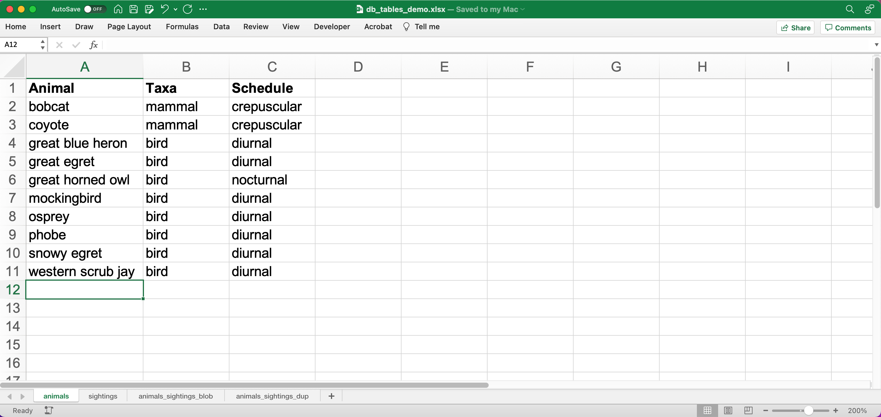
-
The single table breaks down when your data is complex
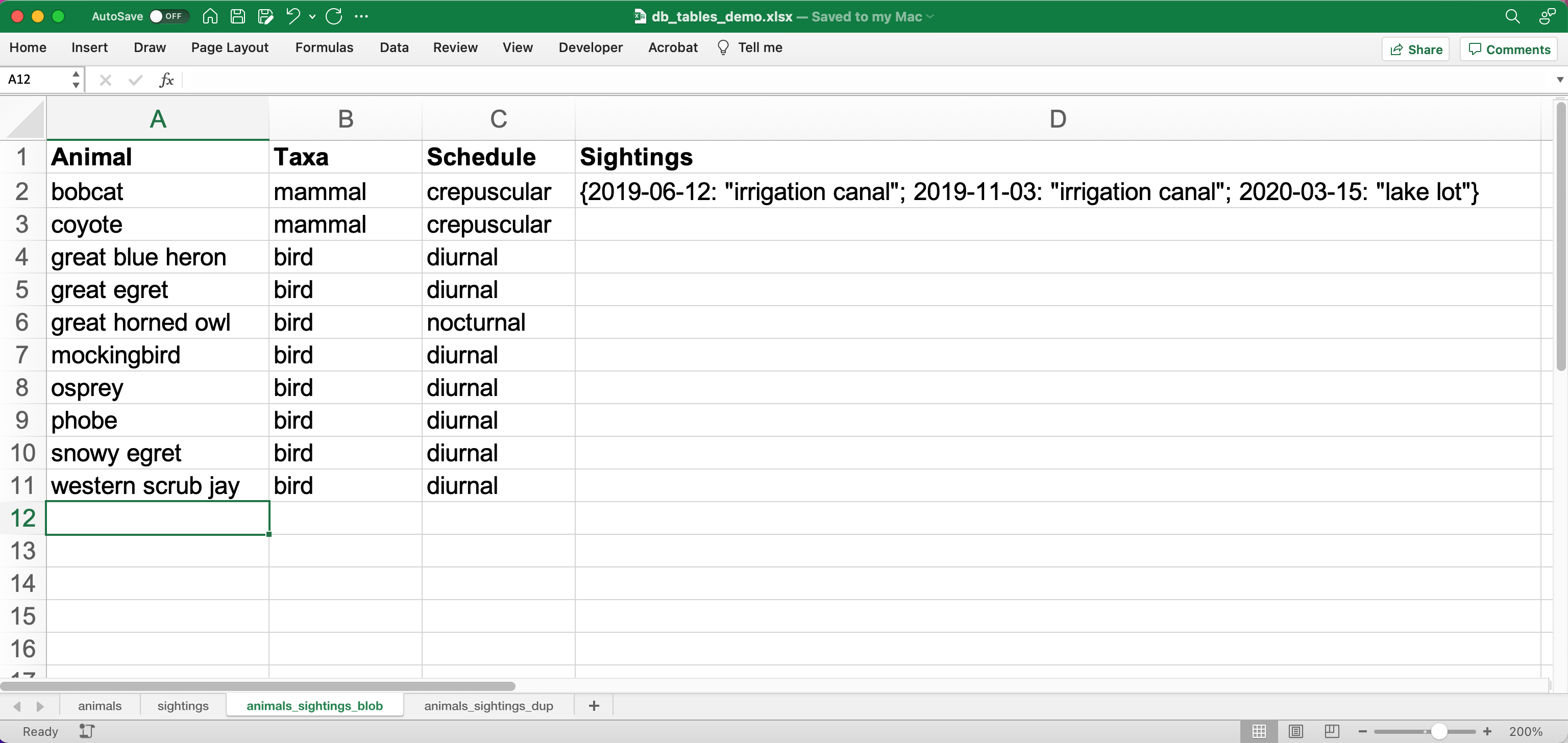
If you use a nested representation, the individual table cells are no longer atomic. The tool for query, search, or perform analyses rely on the atomic structure of the table, and they break down when the cell contents are complex.
-
Complex data with duplicate row
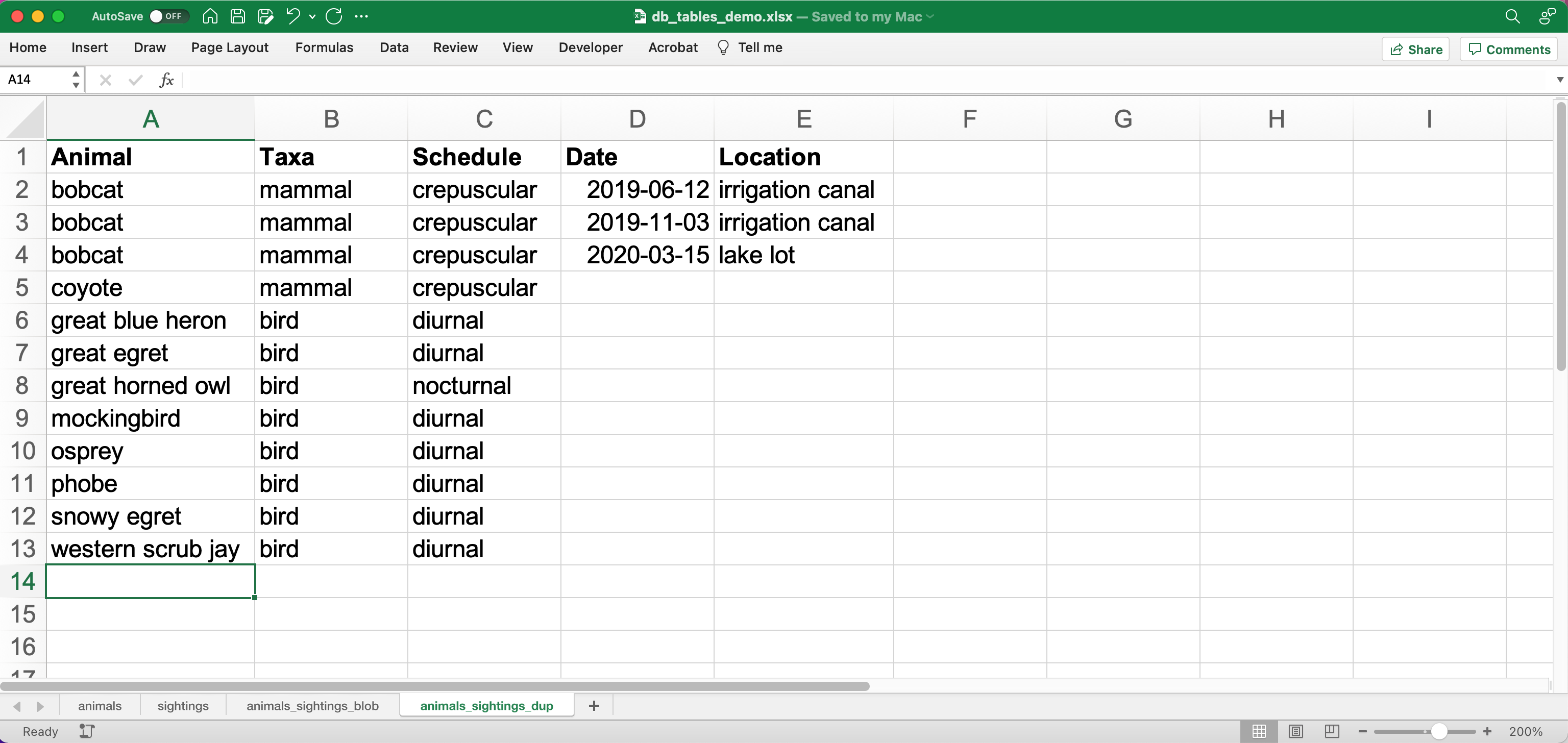
- Storing redundant information has storage costs
- Redundant rows violate the Don't Repeat Yourself [DRY] principle. Every copy is an opportunity to introduce errors or inconsistencies into the data.
- Storing multidimensional data in a single table increases the chance that your records will have NULL fields, which will complicate future queries (more on this later)
-
Solution: Normalize the data by breaking it into multiple tables
Animals Sightings 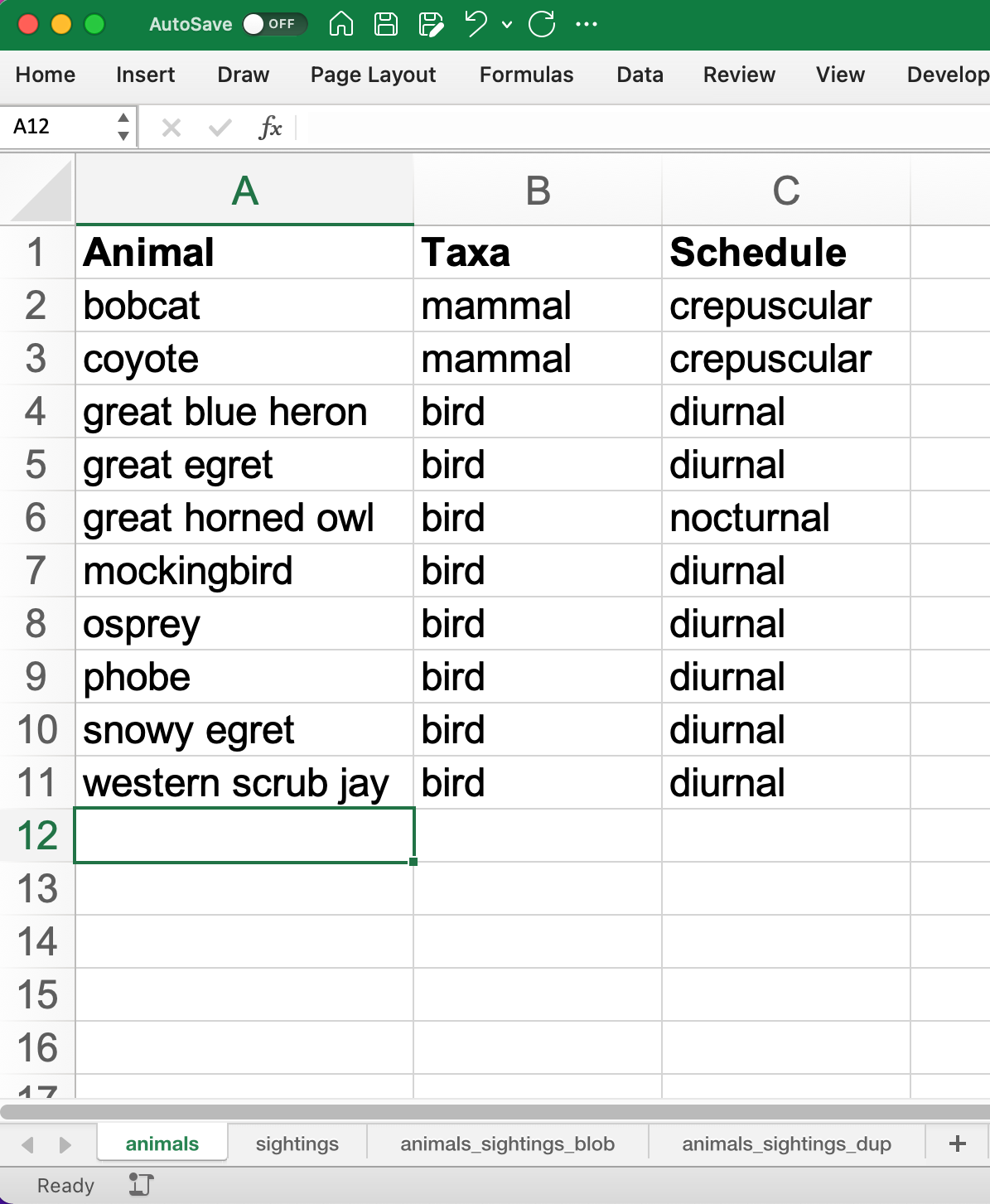
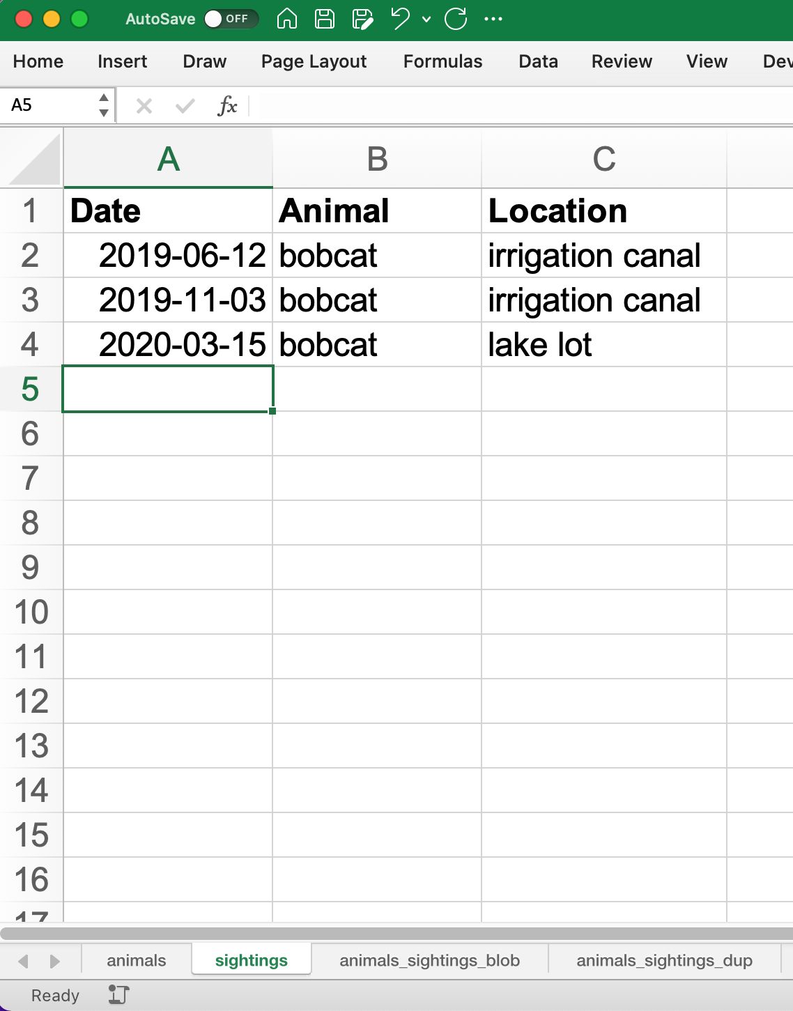
- Every row of every table contains unique information
- Normalization is a continuum. We could normalize this data further, but there is a trade-off in terms of sane table management. Finding the correct trade-off is a matter of taste, judgment, and domain-specific knowledge.
Encode Domain Knowledge
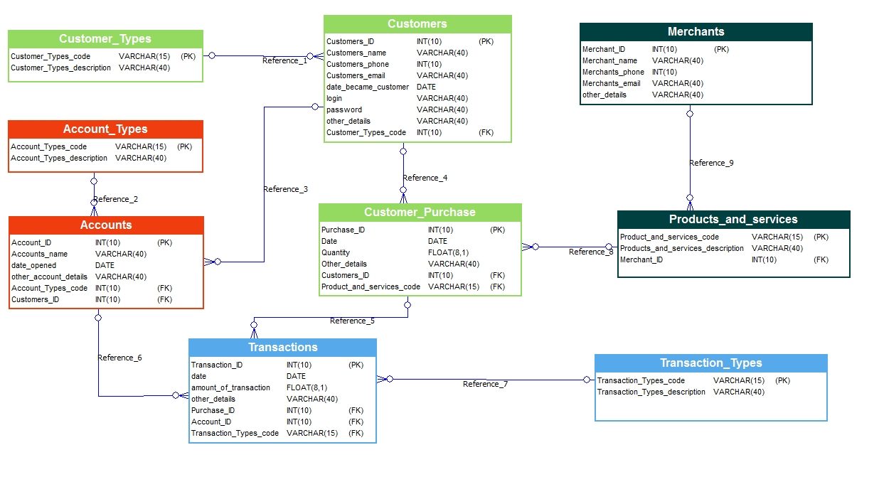
- Encodes shape of domain
- Embeds domain rules: e.g. cannot have a customer transaction without a customer account
- Rules provide additional layer of correctness in the form of constraints
- note that forbidding NULL seems much more reasonable in this context!
Extensions
- Functions
- Data types (GIS, JSON, date/time, searchable document, currency…)
- Full-text search
Accessing data with queries
Basic queries
-
Select everything from a table
SELECT * FROM surveys; -
Select a column
SELECT year FROM surveys; -
Select multiple columns
SELECT year, month, day FROM surveys; -
Limit results
SELECT * FROM surveys LIMIT 10; -
Get unique values
SELECT DISTINCT species_id
FROM surveys;
-- Return distinct pairs SELECT DISTINCT year, species_id FROM surveys; -
Calculate values
-- Convert kg to g SELECT plot_id, species_id, weight/1000 FROM surveys; -
SQL databases have functions
SELECT plot_id, species_id, ROUND(weight/1000, 2)
FROM surveys;
Filtering
-
Filter by a criterion
SELECT *
FROM surveys
WHERE species_id='DM';
SELECT * FROM surveys WHERE year >= 2000; -
Combine criteria with booleans
SELECT *
FROM surveys
WHERE (year >= 2000) AND (species_id = 'DM');
SELECT * FROM surveys WHERE (species_id = 'DM') OR (species_id = 'DO') OR (species_id = 'DS');
Challenge 1
Get all of the individuals in Plot 1 that weighed more than 75 grams, telling us the date, species id code, and weight (in kg).
Building complex queries
Use sets ("tuples") to condense criteria.
SELECT *
FROM surveys
WHERE (year >= 2000) AND (species_id IN ('DM', 'DO', 'DS'));
Sorting
-
Sort by a column value
SELECT * FROM species ORDER BY taxa ASC; -
Descending sort
SELECT * FROM species ORDER BY taxa DESC; -
Nested sort
SELECT *
FROM species
ORDER BY genus ASC, species ASC;
Challenge 2
Write a query that returns year, species_id, and weight in kg from the surveys table, sorted with the largest weights at the top.
Order of execution
Queries are pipelines 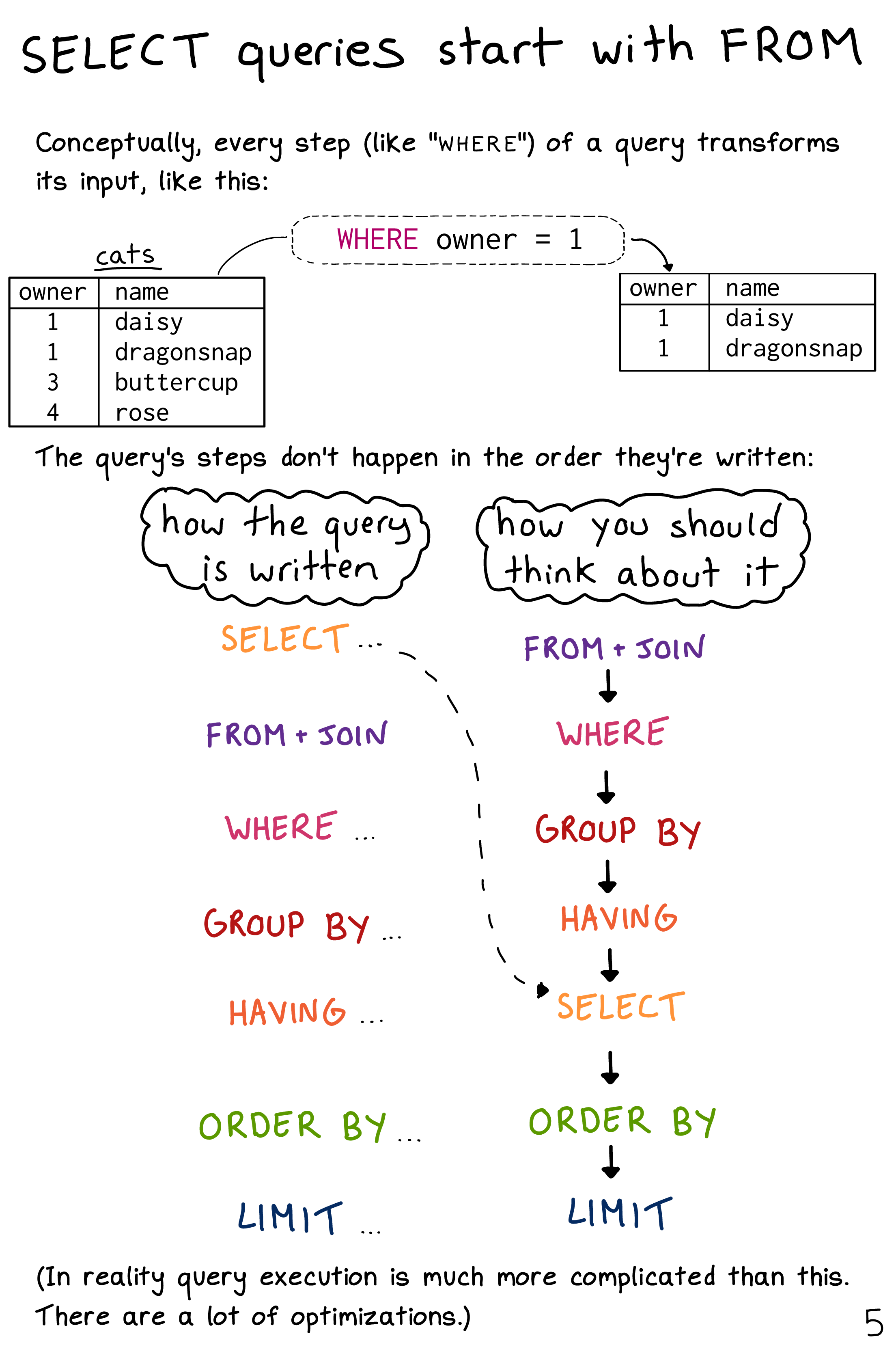
Aggregating and grouping data (i.e. reporting)
COUNT
SELECT COUNT(*)
FROM surveys;
-- SELECT only returns non-NULL results
SELECT COUNT(weight), AVG(weight)
FROM surveys;
Challenge 3
- Write a query that returns the total weight, average weight, minimum and maximum weights for all animals caught over the duration of the survey.
- Modify it so that it outputs these values only for weights between 5 and 10.
GROUP BY (i.e. summarize, pivot table)
-
Aggregate using GROUP BY
SELECT species_id, COUNT(*) FROM surveys GROUP BY species_id; -
Group by multiple nested fields
SELECT year, species_id, COUNT(*), AVG(weight)
FROM surveys
GROUP BY year, species_id;
Ordering aggregated results
SELECT species_id, COUNT(*)
FROM surveys
GROUP BY species_id
ORDER BY COUNT(species_id) DESC;
Aliases
Create temporary variable names for future use. This will be useful later when we have to work with multiple tables.
-
Create alias for column name
SELECT MAX(year) AS last_surveyed_year FROM surveys; -
Create alias for table name
SELECT *
FROM surveys AS surv;
The HAVING keyword
-
WHEREfilters on database fields;HAVINGfilters on aggregationsSELECT species_id, COUNT(species_id) FROM surveys GROUP BY species_id HAVING COUNT(species_id) > 10; -
Using aliases to make results more readable
SELECT species_id, COUNT(species_id) AS occurrences FROM surveys GROUP BY species_id HAVING occurrences > 10; -
Note that in both queries,
HAVINGcomes afterGROUP BY. One way to think about this is: the data are retrieved (SELECT), which can be filtered (WHERE), then joined in groups (GROUP BY); finally, we can filter again based on some of these groups (HAVING).
Challenge 4
Write a query that returns, from the species table, the number of species in each taxa, only for the taxa with more than 10 species.
SELECT taxa, COUNT(*) AS n
FROM species
GROUP BY taxa
HAVING n > 10;
Saving queries for future use
A view is a permanent query; alternatively, it is a table that auto-refreshes based on the contents of other tables.
-
A sample query
SELECT * FROM surveys WHERE year = 2000 AND (month > 4 AND month < 10); -
Save the query permanently as a view
CREATE VIEW summer_2000 AS SELECT * FROM surveys WHERE year = 2000 AND (month > 4 AND month < 10); -
Query the view (i.e. the query results) directly
SELECT *
FROM summer_2000
WHERE species_id = 'PE';
NULL
Start with slides: NULLs are missing data and give deceptive query results. Then demo:
-
Count all the things
SELECT COUNT(*) FROM summer_2000; -
Count all the not-females
SELECT COUNT(*) FROM summer_2000 WHERE sex != 'F'; -
Count all the not-males. These two do not add up!
SELECT COUNT(*) FROM summer_2000 WHERE sex != 'M'; -
Explicitly test for NULL
SELECT COUNT(*)
FROM summer_2000
WHERE sex != 'M' OR sex IS NULL;
Combining data with joins
(Inner) joins
-
Join on fully-identified table fields
SELECT * FROM surveys JOIN species ON surveys.species_id = species.species_id; -
Join a subset of the available columns
SELECT surveys.year, surveys.month, surveys.day, species.genus, species.species FROM surveys JOIN species ON surveys.species_id = species.species_id; -
Join on table fields with identical names
SELECT *
FROM surveys
JOIN species
USING (species_id);
Challenge 5
Write a query that returns the genus, the species name, and the weight of every individual captured at the site.
SELECT species.genus, species.species, surveys.weight
FROM surveys
JOIN species
ON surveys.species_id = species.species_id;
Other join types
Slides: Talk about the structure of joins
Combining joins with sorting and aggregation
SELECT plots.plot_type, AVG(surveys.weight)
FROM surveys
JOIN plots
ON surveys.plot_id = plots.plot_id
GROUP BY plots.plot_type;
(Optional) Challenge 6
Write a query that returns the number of animals caught of each genus in each plot. Order the results by plot number (ascending) and by descending number of individuals in each plot.
SELECT surveys.plot_id, species.genus, COUNT(*) AS number_indiv
FROM surveys
JOIN species
ON surveys.species_id = species.species_id
GROUP BY species.genus, surveys.plot_id
ORDER BY surveys.plot_id ASC, number_indiv DESC;
(Optional) Functions COALESCE and NULLIF
-
Replace missing values (NULL) with a preset value using COALESCE
SELECT species_id, sex, COALESCE(sex, 'U') FROM surveys; -
Replacing missing values allows you to include previously-missing rows in joins
SELECT surveys.year, surveys.month, surveys.day, species.genus, species.species FROM surveys JOIN species ON COALESCE(surveys.species_id, 'AB') = species.species_id; -
NULLIF is the inverse of COALESCE; you can mask out values by converting them to NULL
SELECT species_id, plot_id, NULLIF(plot_id, 7)
FROM surveys;
(Optional) SQLite on the command line
Basic commands
sqlite3     # enter sqlite prompt
.tables     # show table names
.schema     # show table schema
.help       # view built-in commands
.quit
Getting output
-
Formatted output in the terminal
.headers on
.help mode
.mode column
SELECT * FROM species WHERE taxa = 'Rodent'; -
Output to .csv file
.mode csv
.output test.csv
SELECT * FROM species WHERE taxa = 'Rodent';.output stdout
(Optional) Database access via programming languages
R language bindings
-
Resources
-
Import libraries
library("DBI") library("RSQLite") -
FYI, use namespaces explicitly
con <- DBI::dbConnect(RSQLite::SQLite(), "../data/portal_mammals.sqlite") -
Show tables
dbListTables(con) -
Show column names
dbListFields(con, "species") -
Get query results at once
df <- dbGetQuery(con, "SELECT * FROM surveys WHERE year = 2000") head(df) -
Use parameterized queries
df <- dbGetQuery(con, "SELECT * FROM surveys WHERE year = ? AND (month > ? AND month < ?)", params = c(2000, 4, 10)) head(df) -
Disconnect
dbDisconnect(con)
(Optional) What kind of data storage system do I need?
Non-atomic write; sequential read
- Files
Single atomic write (database-level lock); query-driven read
- SQLite
- Microsoft Access
Multiple atomic writes (row-level lock); query-driven read
- PostgreSQL: https://www.postgresql.org
- MySQL/MariaDB
- Oracle
- Microsoft SQL Server
- …etc.
(Optional) Performance tweaks and limitations
Getting the most out of your database
- Use recommended settings, not default settings
- Make judicious use of indexes
- Use the query planner (this will provide feedback for item 2)
- Cautiously de-normalize your schema
Where relational databases break down
- Very large data (hardware, bandwidth, and data integration problems)
- Distributed data (uncertainty about correctness)
Why are distributed systems hard?
- CAP theorem
- In theory, pick any two: Consistent, Available, Partition-Tolerant
- In practice, Consistent or Available in the presence of a Partition
- Levels of data consistency
- Fallacies of distributed computing
- The network is reliable
- Latency is zero
- Bandwidth is infinite
- The network is secure
- Topology doesn't change
- There is one administrator
- Transport cost is zero
- The network is homogeneous
Endnotes
Credits
- Data management with SQL for ecologists: https://datacarpentry.org/sql-ecology-lesson/
- Databases and SQL: http://swcarpentry.github.io/sql-novice-survey/ (data hygiene, creating and modifying data)
- Simplified bank account schema: https://soft-builder.com/bank-management-system-database-model/
- Botanical Information and Ecology Network schema: https://bien.nceas.ucsb.edu/bien/biendata/bien-3/bien-3-schema/
References
- C. J. Date, SQL and Relational Theory: https://learning.oreilly.com/library/view/sql-and-relational/9781491941164/
- Common database mistakes: https://stackoverflow.com/a/621891
- Fallacies of distributed computing: https://en.wikipedia.org/wiki/Fallacies_of_distributed_computing
Data Sources
- Portal Project Teaching Database: https://figshare.com/articles/dataset/Portal_Project_Teaching_Database/1314459 Specifically, portal_mammals.sqlite: https://figshare.com/ndownloader/files/11188550